Deep Upscaling
Jul 10, 2022
Click the video for the live demo hosted on Shadertoy.
Image upscaling is the process of synthesising a super-resolution image from a low-resolution prior. The most basic upscaling algorithms are simple piecewise interpolation schemes (bilinear, bicubic, etc.) which blend adjacent pixel values at the cost of bias and aliasing. More sophisticated techniques use edge detectors, diffusion or regression to intelligently reconstruct high-frequency detail. Though superior to naive interpolation, they still perform relatively poorly given that they usually consider only the local neighbourhood of pixel values.
Over the past few years, the rapid advance of deep learning learning has transformed the field of image processing. When properly trained, a deep neural network is can convincingly hallucinate missing details from even the most degraded of images.
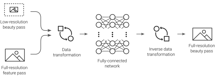
This demo aims to implement an end-to-end workflow of a simple upscaling pipeline powered by a deep neural network. First, a low-resolution beauty pass is rendered together with a native-resolution feature pass of a 3D scene. Feature data is generally very cheap to render so the additional of rendering two passes still considerably lower than rendering out the beauty at its native resolution.
Next, the shader constructs a data set which is transformed to remove the DC component before being fed into a multi-layer perceptron (MLP). The model is then progressively trained using stochastic gradient descent to adjust the weights and biases. Finally, the network is evaluated over the low-resolution beauty pass, upscaling it back to its native resolution.
Rendering
Since Monte Carlo path tracers offer an unlimited source of high-quality training data, I looked to simple looping animation from one of my generative art projects for inspiration.
A paired-down version of this generative scene is used to synthesise the training data. Click to see the real-time demo on Shadertoy.

The original scene consists of a polyhedron rotating around a point light and immersed inside a sparse volumetric medium. Volume sampling along the ray creating characteristic light rays to emanate from the center of the object. Given the relatively tiny size of the MLP, I stripped the scene down even further so that the model is effectively only training on edges and simple curves. I also configured the renderer to output a normalised depth map derived from the camera ray hit distance.
Model Architecture
One of the principle challenges with implementing a fully-connected network within the frame buffer of a shader is the sheer number of parameters that have to be juggled during training. An additional bottleneck is the refresh rate which in Shadertoy is capped to 60fps. This meant that in order to train the model within a reasonable amount of time, I was forced to favour large batch sizes at the expense of having fewer parameters.
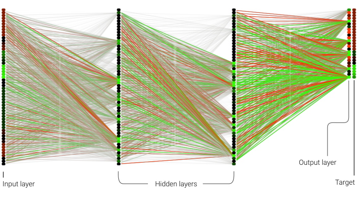
The complete graph of the weights and activations of the multilayer perceptron. The output layer also includes the target from the training set for visual comparison.
To upscale a single pixel, the model ingests two kernels containing the transformed beauty and depth data sampled from the local neighbourhood. Each kernel is a 5x5 pixel grid making for a total width of 50 neurons per layer. I used two full-width hidden layers and one half-width output layer representing the upscaled kernel, making for a grand total of 6,400 trainable parameters. Leaky ReLU was used as the activation for all layers and a vanilla L1 norm for the loss function.
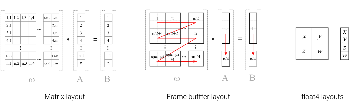
The correspondence between the layout of the matrix (left) and the location of the data in memory (center and right). Click to enlarge.
The network parameters are arranged in memory so as to minimise the number of texture taps during matrix multiplications. The diagram above illustrates the ordering of the elements of an n x m matrix. Weights are packed so that each float4 pixel straddles two rows and two columns of the corresponding matrix. The n x 1 matrices representing the biases and neuron activations are packed contiguously since each only has a single column. During the inner loop of the multiplication operation, 4 quads full of weights and 4 quad containing the activation or error are loaded and multiplied together. This is efficient since it means computing the matrix transpose is no more expensive than during the forward pass.
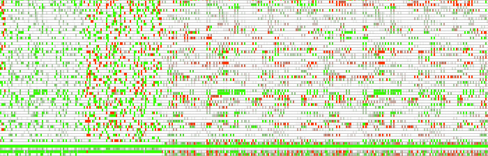
A raw visualisation of the model as laid out in texture memory.
Each layer in the network consists of 4 matrices: weights, biases, activations and errors. An additional data block encodes auxiliary information including the sample loss as well as input and output data used during training. Together these data comprise a single training target with batches of targets being trained on simultaneously. A frame buffer at the default resolution of 1,200 x 675 has approximately 3.2 million full-precision parameters making for an effective batch size of roughly 500 elements.
Dataset Generation
Generating a dataset on which the MLP can train requires generating a set of patches that encapsulate both the source and target functions. Randomly selecting patches across both spatial and temporal domains initially yielded poor results given that most of the samples ended up landing in uniform or uninteresting areas. This resulted in the model underfitting to the data and subsequently failing to preserve edges and discontinuities.
To address this problem, I added an additional quality control step in which the gradient of the patch is measured and used as a heuristic to decide whether or not it should be added to the training set. The larger the gradient, the more likely the patch is to be accepted. Rejected patches are reset and subsequently regenerated using a different random position. By carefully tuning the acceptance criteria, I was able to get the model to respond more effectively to high-frequency details in the signal.
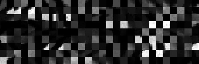
The training set swatch. Each triplet of tiles corresponds to the low resolution beauty pass, the full resolution feature pass and the full resolution beauty pass respectively.
Another major issue was the dominance of the DC frequency in each patch. Using the raw data from the renderer caused the network to learn the direct relationship in brightness between input and output, thereby making it behave like a simple bilinear filter. This was fixed by subtracting the mean value of the signal from every element in the patch and applying a gamma ramp to further boost the residual signal. This transformation is similar in essence to a Laplacian pyramid or wavelet transform since it isolates the components of the signal that the network needs to learn.
Training
Given the non-linear flow of data through a neural network, I found it necessary to use the shader’s frame counter as a clock to synchronise training operations across each epoch.
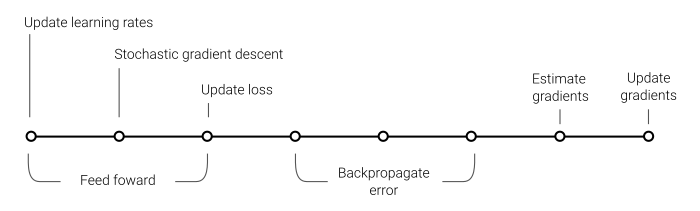
For the set of hyperparameters chosen for this model, a single epoch requires 8 frames to complete (assuming the entire training set fits into the frame buffer). First, the input data are fed forward through the network followed by the loss and residual error being calculated and stored. Next, the error is back-propagated before the gradients are calculated for each member in the batch. Finally, the gradients are integrated and the individual batch gradients updated. The concurrent nature of the batching process means that certain operations can be done in parallel. For example, updating the learning rate and applying gradient descent can be done at the same time as the forward propagation step, reducing redundancy as well as training time.
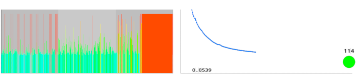
Per-weight learning rates (left) and a plot of the L1 loss function (right). Also shown is the total epoch counter (bottom right).
Given the limited amount of space available in the framebuffer, I decided not to create a validation set and instead devote all the space to the training set. As a result there is no quantitative measure of the model’s performance, however the fact that the quality of the results are ultimately assessed from the upscaled output means that this is no big loss.
Inference
Inference is performed continually while the network is training, so the output from the model can be visualised in real-time. After around 500 epochs, the network converges to the point that most residual artifacts have almost completely disappeared from the output.

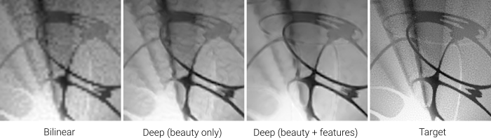
Close-up comparisons between bi-linear upscaling (left) and deep upscaling (right). The model was trained for 500 epochs with an L1 loss.
Given the small size of the network and training set together with the reduced training time, I think these results are relatively good. A better loss function (e.g. using SIREN’s first and second order derivatives) would almost certainly find a more optimised latent space. In addition, one of the many kernel-predicting models would also likely perform better.
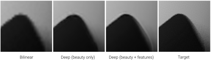
I also tried some basic ablation testing by zeroing out the inputs containing the full-resolution feature data. Somewhat surprisingly, the model still managed to do a reasonable job, particularly near high-amplitude, high-frequency details. This was interesting as I honestly expected it to fail completely given that I was asking it to up-res the prior by 3x while only using a 5x5 kernel as input.
Additional Results
While the spinning tetrahedron works well as a canonical test case, it’s geometric simplicity doesn’t adequately test the limits of the MLP for this sort of rendering problem. To test the capacity of the network to learn the complete feature set of an animated sequence, I swapped in two additional scenes that exhibit much higher geometric complexity and shading effects that are not captured by the feature buffer.
Click the video to see the live demo on Shadertoy.
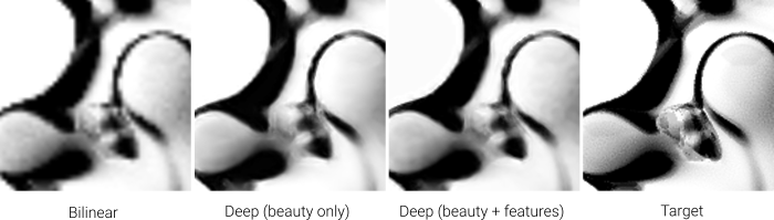
In the examples above, the tetrahedron has been substituted for a swarm of “meta-toruses”, isosurfaces of the charged potential field of a ring singularity. Unlike with the tetrahedron, the upscaler struggled to reconstruct most of the sub-pixel detail without the assistance of the full-resolution feature buffer. That said, I was once again impressed at how well this worked considering the relatively small number of parameters in the model.
Click the video to see the live demo on Shadertoy.
For the second test, I tried recreating a water-like effect using metaballs rendered with a liquid shader. Here, the feature buffers do almost nothing to improve the quality of the reconstruction, however this was almost certainly to do with the fact that the patterns that flow and shift across the surface are not represented adequately in either the training data nor indeed in the model itself. Using different auxiliary features such as surface normals or albedo would likely improve these results considerably.
Project Links